
Note that all images can be enlarged with a mouse click.
Above is one possible scenario for future output from the Bakken which suggests a total cumulative output of 7 billion barrels (Gb) from 1953 to 2073. Current US crude oil inputs to refineries is about 15 million barrels per day (52 week average above 14.9 MMb/d for past 6 months) which is 5.475 Gb per year, the total Bakken output of 7 Gb would supply current refinery inputs for 1.27 years. When we account for the 0.57 Gb of Bakken which has been produced we are left with about 1.2 years of crude inputs at current levels.
The above estimate is based on a presentation from the North Dakota Industrial Commission (NDIC) Oil and Gas Division (see slides 25 to 30). This presentation suggests about 41,000 wells will be drilled in the Bakken at a rate of 1500-3000 wells per year, I chose 2460 wells per year and a total of 42,000 wells drilled by Sept 2028.

The model is based on the average well profiles above. The well profile from Dec 2004 to Dec 2007 is 50 % of the well profile from Jan 2008 to Jan 2013. From Feb 2013 to Sept 2028 the average well profile decreases by 1 % each month or 12.4 % per year. There are over 180 separate well profiles between 2013 and 2028, I have presented 2 in the chart above (Jan 2018 and Jan 2023). The 30 year estimated ultimate recovery(EUR) is 303.5 kb, 166 kb, and 91.8 kb in Jan 2013, 2018, and 2023 respectively. In Jan 2018 the EUR is 55 % of Jan 2013, in Jan 2023 it falls to 30 % and by Jan 2028 it is 17 % of Jan 2013. This compares with a 30 year EUR of 570 kb for the NDIC typical well and for Mason's model (PDF, see pp5-6, but note that data in figure 5 is incorrect) the 30 year EUR is 500 kb (using Di=0.197, b=1.4, and qi=14,225 and the Arps hyperbolic equation on p 6). The hyperbolic model of the "Bakken Average Well" uses Di=0.19, b=0.95, and qi=14,225. Based on Arps, b should be between 0 and 1, not 1.1 and 1.4 as Mason suggests, for b>=1 the EUR is unbounded (infinite) as time appoachs infinity.


Each of these plots uses the average well profiles presented previously in combination with Bakken historical data from the NDIC, the model matches the data fairly well from 2007 to 2013.
If we substitute the NDIC typical well or Mason's model for the "average Bakken well" we find:

If we extend these using my original scenario:
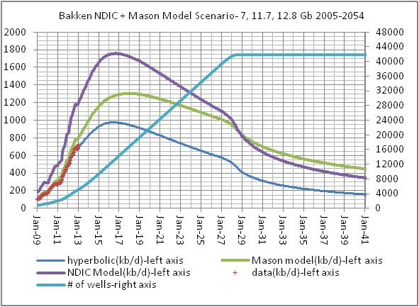
The lowest of these three curves matches the data much better than the NDIC Typical Well or the model presented in James Mason's paper. As a side note, the NDIC typical well matches a hyperbolic with qi=27500, Di=0.19, and b=0.95(see chart below), the hyperbolic matching the data uses the same qi as Mason's model, but uses the Di, and b matching the NDIC typical well, so it is a hybrid of the two.

Finally the model presented in the first chart is rescaled so that it can be more easily compared with scenarios presented in previous posts. Most of these scenarios had a less rapid decrease in productivity of the average well after Jan 2013 (usually 0.5 % each month or 6 % per year). The earlier scenarios also increased the number of new wells more rapidly and topped out at a rate of 3000 new wells per year, the model below reaches 2460 new wells per year (205 per month) in June 2016 and remains at that level for 10 years.

We will explore a few variations in future scenarios in an upcoming post.
DC
DC, Amazing prediction you made considering the recent USGS report:
ReplyDeletehttp://www.theoildrum.com/node/9977#comment-960532
I placed this on TOD yesterday to see the reaction. No comments yet.
WHT,
DeleteThe USGS predicted 7.4 BBO, mostly from North Dakota and Montana, the North Dakota portion is what I am attempting to model (using NDIC data) and that portion has a mean estimate of 5.8 BBO (billion barrels of oil).
DC
DC
ReplyDeleteI read Mason's article in the OGJ. And found it detached from reality.
Can you summarize the key error you think he made. You reference it above.
I think you are saying his decline curve had a B exponent larger than 1--which, in effect,
gave him a typical well size larger than 500,000 b, whereas you expect something more like
300k.
Is that the gist of it?
Hi James,
DeleteThe short answer is yes.
I can only guess at what led to a choice of b=1.4 in Mason's paper, I believe he may have been influenced by predictions from the North Dakota Industrial Commission (NDIC) of a 30 year EUR of around 500,000 barrels.
I chose a b exponent between zero and one because that is what the original Arps equations for a hyperbolic decline model suggests and also because the actual oil output according to the NDIC does not match well with Mason's model.
It is interesting that if the initial production is scaled back to about what Mason uses and we use Di and b that match the NDIC typical well profile, we get a model which matches the data pretty well.
DC
James, As we have discovered, these hyperbolic profiles that Mason and others use are very susceptible to integrating to infinite cumulative values.
ReplyDeleteDC has taken pains to give a realistic estimate of what a typical cumulative well size is.
Even estimating the first years production wrong can lead to cumulatives that are off by 150K barrels.
The USGS must be making the same kind of estimate because DC and their ultimate values both come out to around 7 billion barrels.
Mason seems pretty amateurish. You should watch Drilling Info blog. Sometimes some good analyses done and they will reply to comments.
ReplyDeleteThe USGS work suggests a b factor around 1 (with a transition to exponential at some point). I believe gas shale wells have shown b factors above 1 (despite Arps paper). Obviously they don't go to infinity though.
I would still really like some resolution/discussion of the company type curves versus USGS. Maybe there is some explanation. Or maybe if not, interesting to hear them try to justify it.