In my June 14 post I discussed future decreases in average well productivity based on a single average well profile to create scenarios which would match the range of technically recoverable resources (TRR) in a recent USGS estimate for the Bakken/ Three Forks.
A recent discussion at the June 15, 2013 Drumbeat at the Oil Drum was very interesting with Rune Likvern providing great insight (as usual) into recent data on Bakken output in North Dakota.
Mr Likvern believes that we may be seeing a decrease in average well productivity because a simulation with wells added at a rate of 125 well per month from Jan 2013 to April 2013 is showing greater output than recent data with 70 fewer wells added (500 for simulation vs 570 actual). A decrease in average well productivity is one possible explanation. An alternative possibility is that the average well profile may be different from the average well profile that Mr. Likvern has chosen.
I have created various well profiles in an attempt to match James Mason's work, Rune Likvern's work, the NDIC typical well, and the actual production data from the NDIC. I have recently created some newer well profiles by using a minimization of the sum of the squared residuals between the model and data over the period from Jan 2010 to April 2013. When no constraints are put on the minimization we get qi=11070, b=0.41, and d=0.078 (I call this model 7).
In Excel format, q=qi/(POWER((1+b*d*t),(1/b)))
where q is output in barrels/month in month t,
t is months from first output
(I use t=0.5 for my first month and then increase by 1 for future months so that I get mid month output.) The well profiles can be easily reproduced in a spreadsheet.
As an alternative I constrained b to be less than 1 (as originally specified by Arps) and qi=>13750(greater than or equal to 13750) and the solution was qi=13750, b=0.999, d=0.615 (model 6). Mr. Likvern's well profile matches well with qi=14700, b=1.48, d=0.28. Graphically we have:
 |
| Figure 1- Bakken Well Profiles |
For the first 3 years these different well profiles are nearly identical (in terms of cumulative output), after 5 years model 1 can be distinguished from models 6 and 7 and it takes 6.5 years before models 6 and 7 start to show a significant difference.
I have used these profiles and created some new scenarios where it is assumed that up to Dec 2014 there is no decrease in average well productivity and that from May 2013 to Dec 2014 150 net wells are added each month (1800 wells per year).
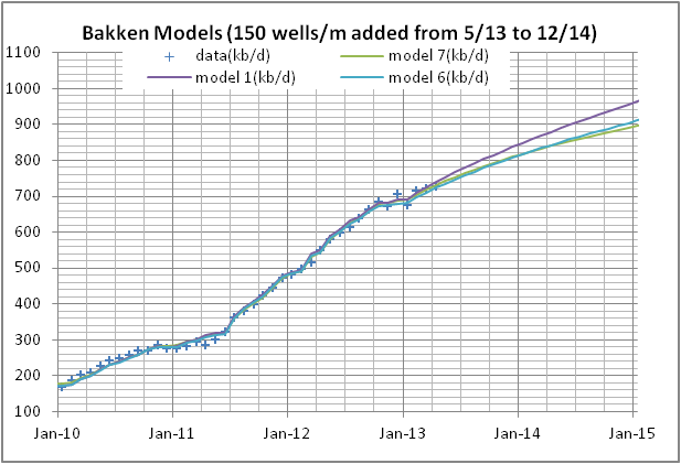 |
| Figure 2 |
All of this got me thinking about my previous post and trying to match the range of USGS estimates from F5 to F95 by varying the decrease in well productivity. Maybe we can do this a little differently and create a single scenario which matches the USGS Mean TRR for model 6 (the middle curve in figure 1). We leave the scenario the same as in figure 2 up to Dec 2014 (no decrease in well productivity up to that point and 150 wells/month 5/13 to 12/14). Then the number of wells per month ramps up to 167/month by April 2016 and remains at that level until we reach 42500 wells in 2032. For model 6 and a Mean TRR of 5.8 BBO well productivity decreases as follows:
 |
| Figure 3 |
We use this same decrease in well productivity for model 1, 6 and 7 to create the following 3 scenarios:
 |
| Figure 4 |
These scenarios do a good job of covering the range of the USGS estimate (3.5 to 9 BBO) and range from 3.6 to 8.8 BBO. I have not attempted to include prices, but may introduce my low price scenario (close to the EIA reference price case) to see how profitability considerations will reduce the URR.
A question for any one in the oil business, how low can we get well completion costs in the Bakken over the next 20 years, is it realistic to assume we can get from $9 million/well down to $4.5 million per well (in Jan 2013 $) by 2033? If not, what number is realistic?
I am hoping to introduce technology into my model and I plan to use well completion costs as a proxy for technological advances.
Edit: 6/18/2013
Many of my previous scenarios used model 3, so I am presenting a comparison of model 6 and 3 where all of the same assumptions were used as in figure 4 above:

DC
DC, you were asking about the fit to this curve:
ReplyDeletehttp://img441.imageshack.us/img441/8193/p8w.gif
Cumulative = 1850/(1+SQRT(150/t))
where t in years.
It was straight dispersive diffusion, no Ornstein-Uhlenbeck
Your Eagle Ford profile has a strong O-U character
https://sites.google.com/site/dc78image/images/efwellpro.png
Cumulative = 2350/(1+SQRT(50/t'))
where t' = (1-EXP(-1.6*t))/1.6
So the EUR cumulative is about the same in both cases.
The effective diffusivity is 3x higher in the second case, but is tempered by a strong reversion to the mean.
Interesting how they differ.
DC, here is the fitted Eagle Ford curve
ReplyDeletehttp://img163.imageshack.us/img163/3246/i4m.gif
Cumulative = 10000/(1+SQRT(105.75/t'))
where t' = (1-EXP(-0.012*t))/0.012
Also shown is a hyperbolic
Cumulative = 255/(1+24/t)
Interesting how a strong O-U diffusive model is close to a hyperbolic. There are subtle differences in the initial slope and in the asymptote.
WHT,
DeleteSorry it took so long for me to reply. Thank you.
I had attempted to use the OU diffusion model for the Bakken and Eagle Ford, but I was having difficulty matching the data of the first 24 months, the OU diffusion model ramps up very quickly over the early time period. I was contemplating using a hybrid hyperbolic/OU Model because I like the fact that the OU Model has a physical basis where the hyperbolic is more of a curve fitting exercise. I decided just using the hyperbolic would be easier, especially because my understanding of the underlying physics of the diffusion process is pretty sketchy and I don't really have any data or parameters for these geological formations which I could use to verify if the various parameters I am using in my OU Model make any physical sense. Essentially It was a choice between two different curve fitting problems, each with three parameters, and the hyperbolic seemed to fit the data better over the first 24 to 36 months (which is all the data I have so far for the Shale plays).
I do understand however that using the physical model has advantages because I could create a scenario using OU diffusion even without a good understanding of the underlying physics and then some one like you could look at it and say no, parameter x, y or z in your model are not even in the ball park, that x would need to be between a and b, y between c and d, and z between e and f, for the model to match the real world.
DC